INTRODUCTION

This lab maps a room by rotating a robot, collecting ToF readings. Quality depends on reading quantity and consistency. Solve it using open loop control, PID on orientation, or PID on angular speed. Merge readings with transformation matrices, plot, and draw the map.

Prelab

Parts Required

• 1 x Fully assembled robot, with Artemis, TOF sensors, and an IMU.

------------------------------------------------------------------------------------------------------------------------

LAB TASKS

Orientation Control

At first, I decided to implement the orientation control for realizing the on-axis rotation as slow as possible, but I encountered the problem that it could not reach the target angle which changed every second.

Open Loop Control

Hence, I used the open loop control for the mapping. The code in the main loop is shown below, where the mapping_on and counter_max determine the process of this rotation. Additionally, the motor will move for 50 ms every 150 ms, in which case the TOF sensor reading can catch up with the control loop.

The following function is to record the current time stamp and the distance, which will be sent to the laptop through BLE.

In case MAPPING, we can obtain the maximum record number through the Python command, and we turn the mapping_on flag on to implement the mapping.

Furthermore, the SENDING_MAPPING_DATA case is established as below:

With all the program organized in the Arduino C code, we can implement the BLE Python function to control the robot rotation of 360 degrees.

This video shows the 360 degrees' rotation of the robot:

Data Analysis

Therefore, we can get the data through the following code:

According to the arena, there are totally five points to measure. With the data obtained, we can plot the diagrams based on time vs tof distance.

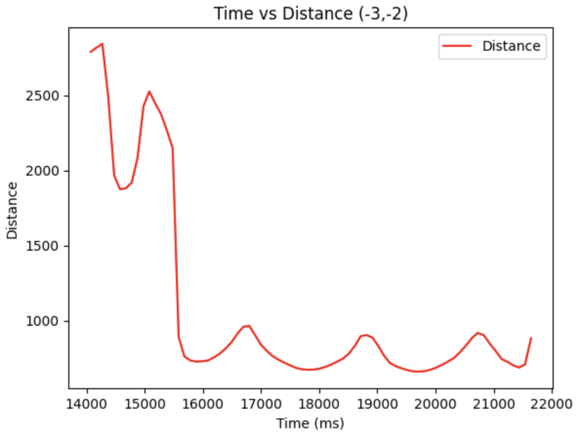
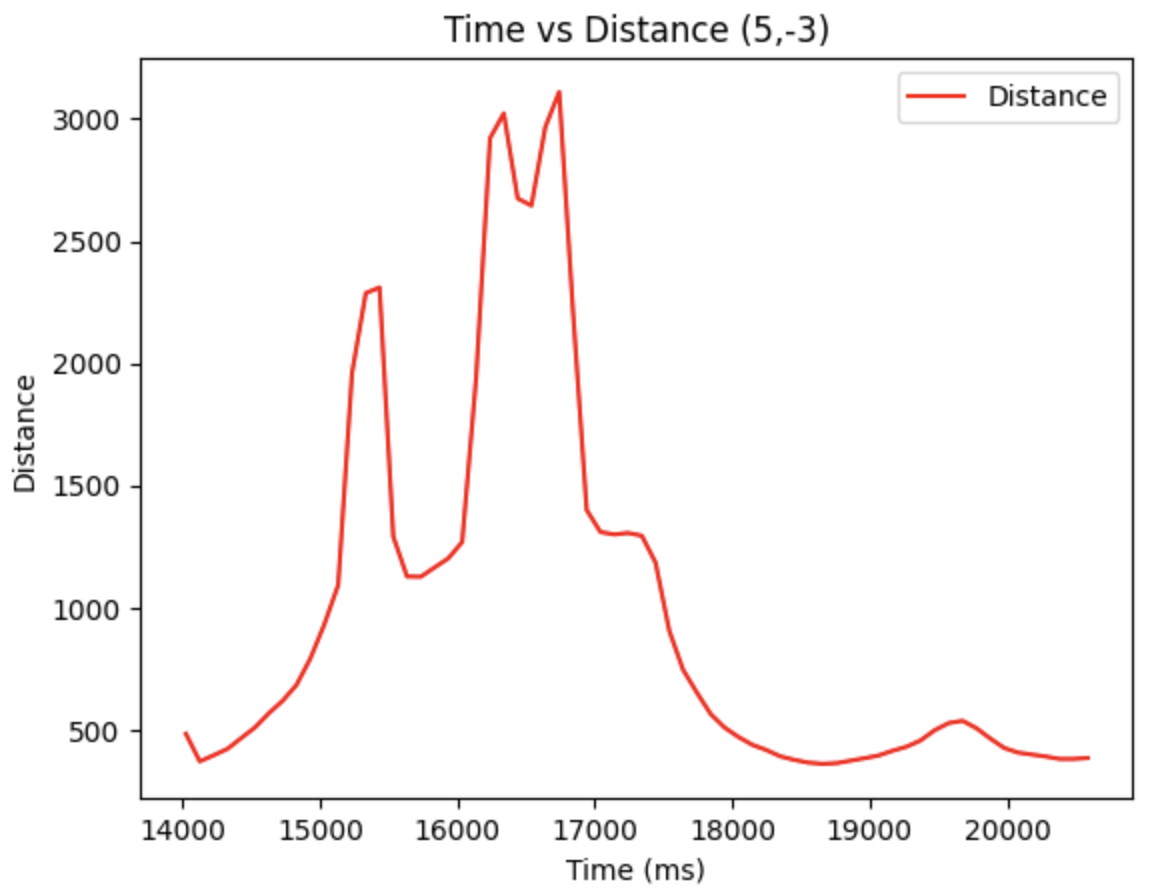
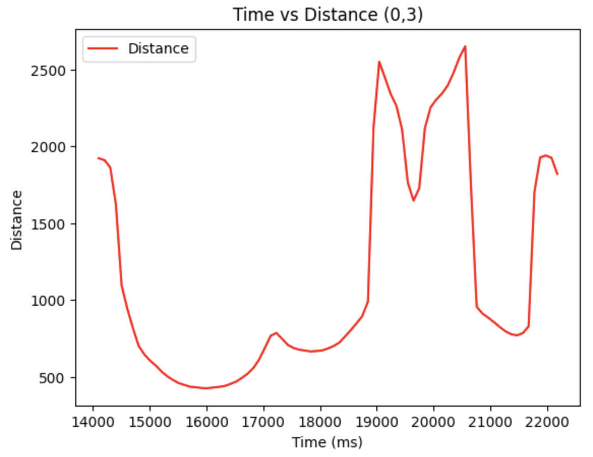
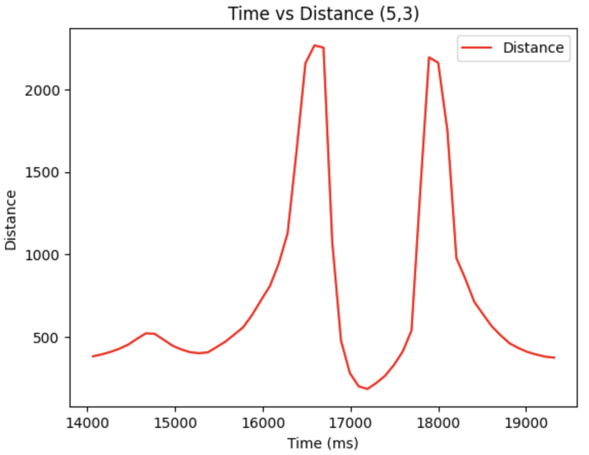
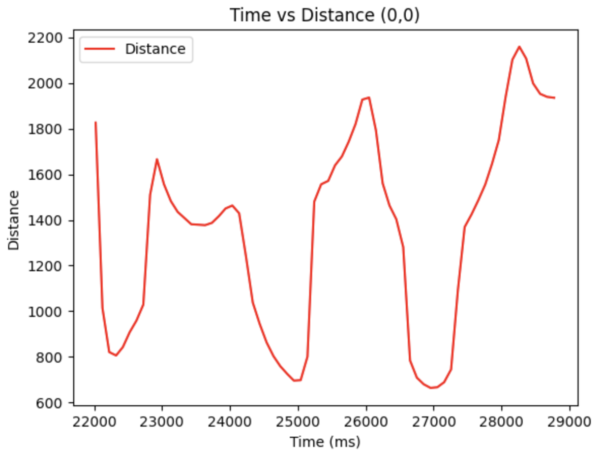
Hence, the polar diagram can be retrieved as below, by using the linespace generation in Numpy library. The euqation for theta is:

theta1 = np.linspace(0, 2*np.pi, (len(mapping_distance1)))

Therefore, we can get the polar diagrams as below:

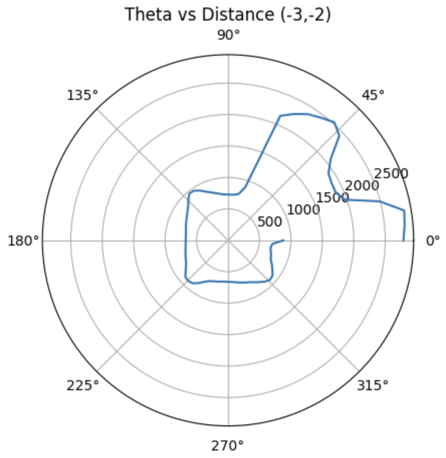
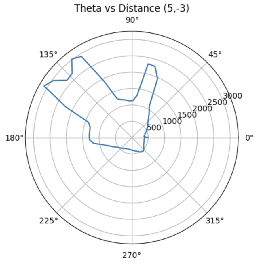
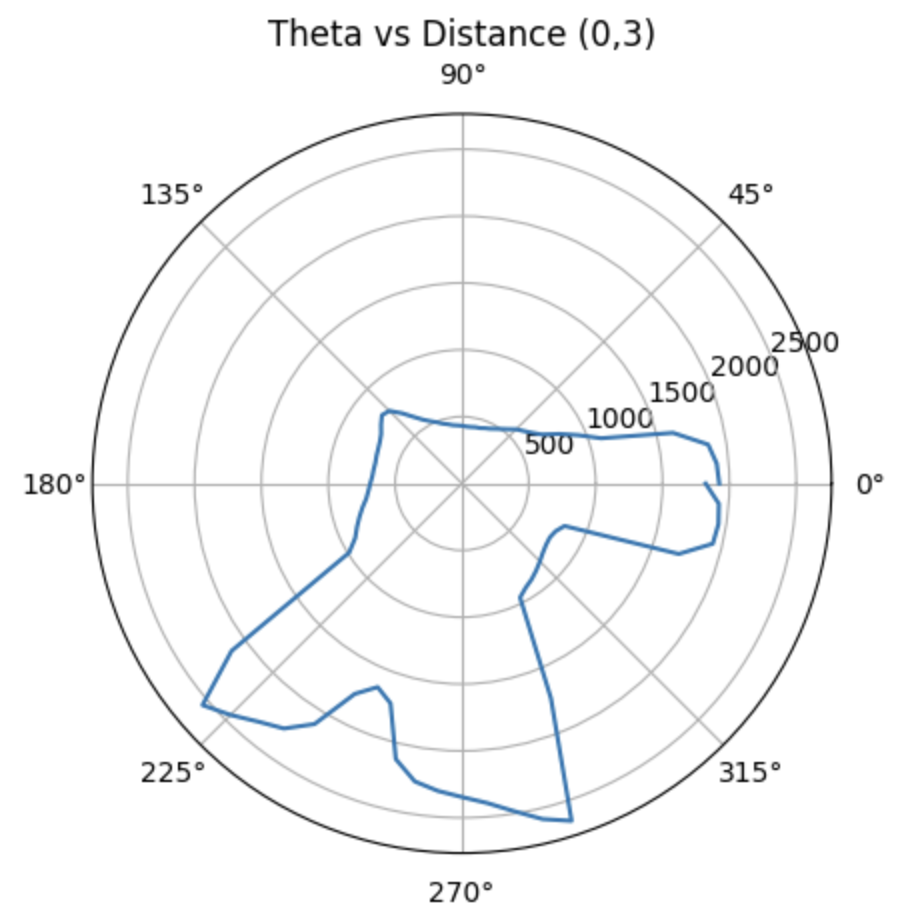
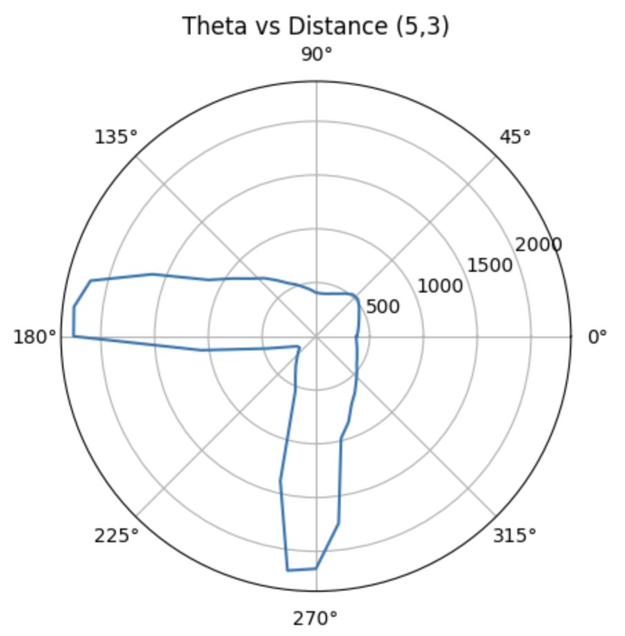
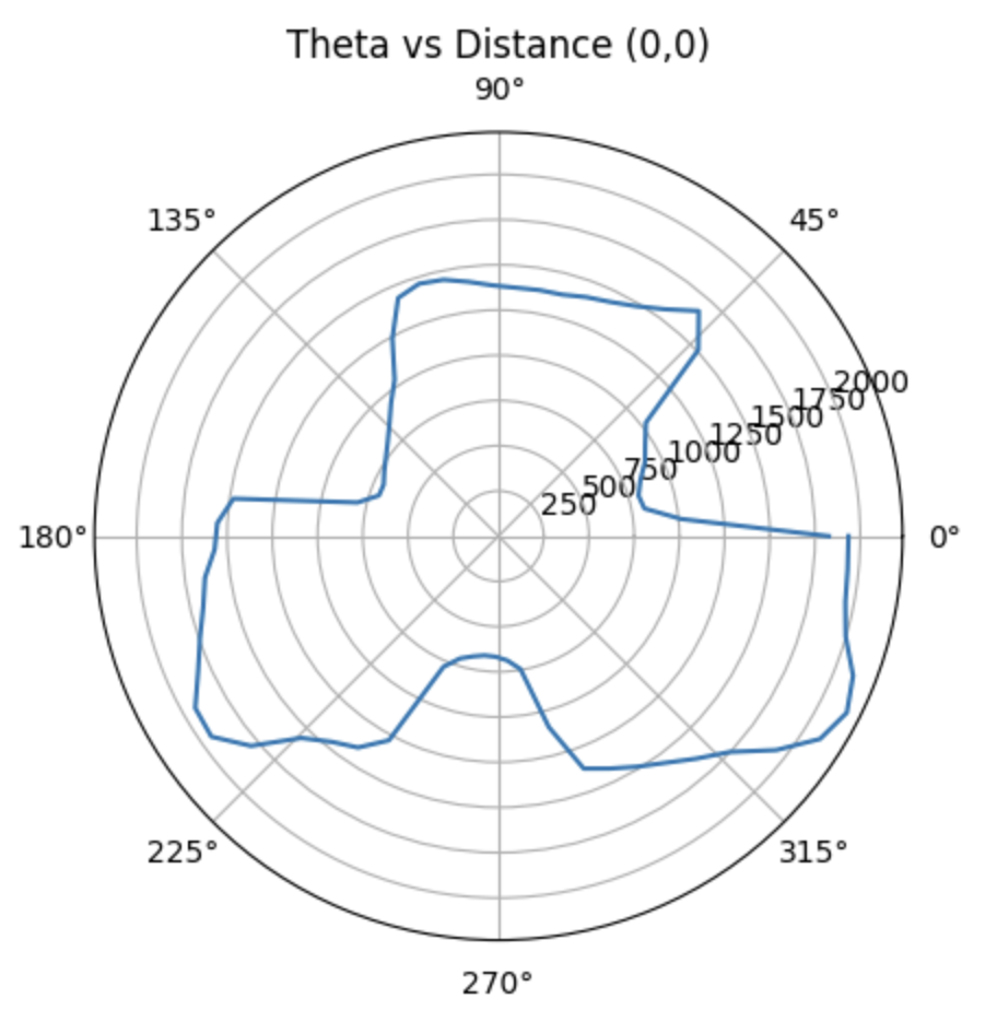
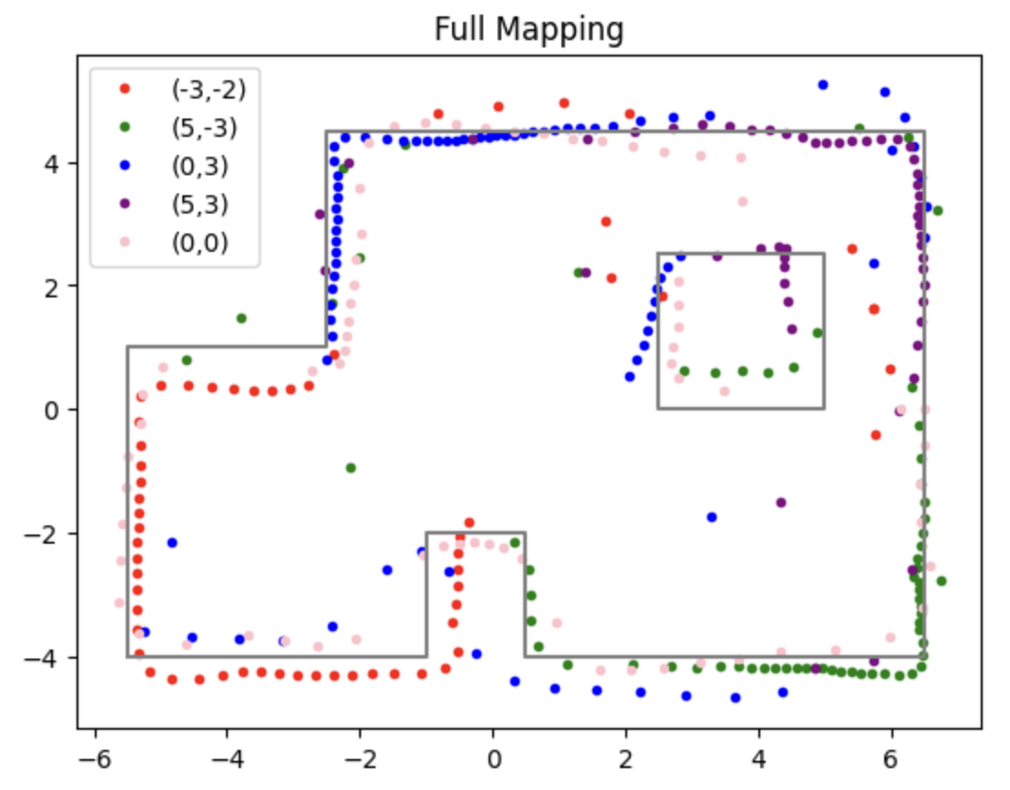
Moreover, with the code below, we are able to obtain the global coordinates of the point plotted in the polar diagrams, where the x_origin and y_origin represent for the coordinate of the rotation point. They are (-3,-2), (5,-3), (0,3), (5,3), (0,0). And the x axis should be adding 50 mm, since the distance of the TOF sensor to the rotation coordinate is approximately 50 mm.

Consequently, the edges of the boxes and the walls can be drawn in the global frame, according to the TOF distance data.

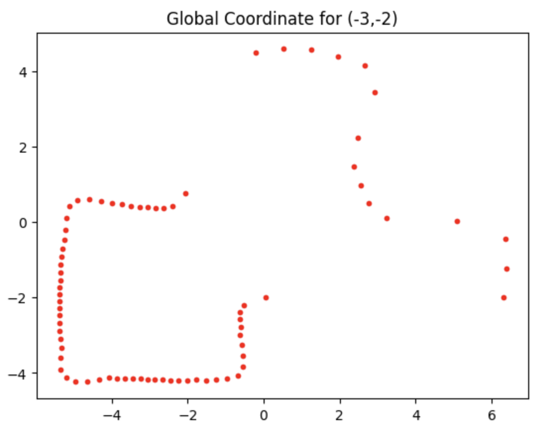
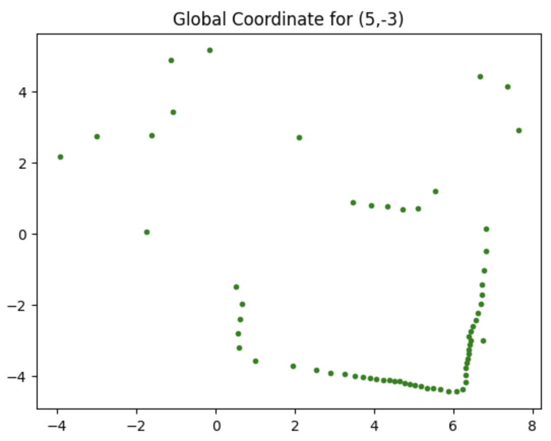
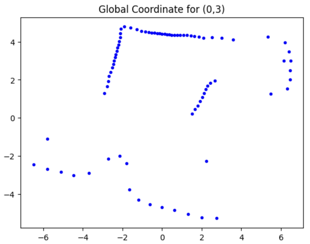
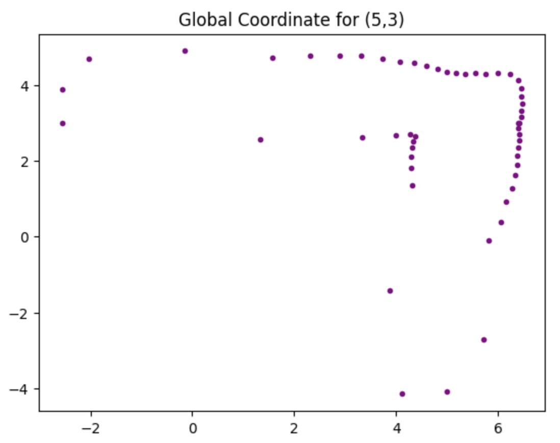
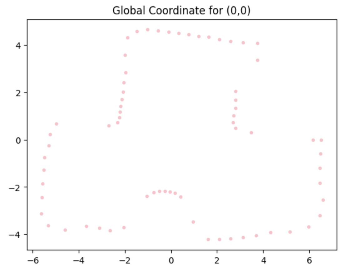
And all those points can be plotted into the same diagram, and compared to the actual edges, which is drawn by the grey lines in the figure.

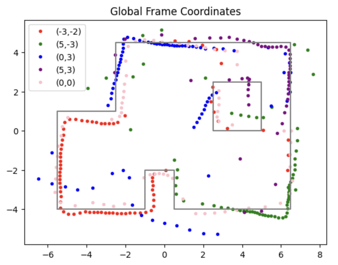
As we can observe from the figure that the mapping point is not exactly aligned with the actual edges, so a little calibration can be implemented to the data we have obtained. In this way, the above diagram can be modified and shown below.

DISCUSSION

This lab effectively mapped a room using a robot equipped with ToF sensors and an IMU. Open-loop control proved successful in rotating the robot for data collection. The collected data were processed, plotted, and transformed into a polar diagram, revealing the room's edges and walls. In the discussion, the accuracy of the mapping results and potential improvements could be addressed.