INTRODUCTION

This lab section is to setup the IMU, getting the accelerometer and gyroscope data. Furthermore, the low pass filter and complimentary filter can be applied to ensure the accuracy and stability of the system. Finally, the sampling function can be added into the main loop to store the data and then transmitted to the laptop through Bluetooth.

SETUP THE IMU

In this section, it is required to setup the IMU. With the knowledge of accelerometer and gyroscope, we can modify the code to realize the accuracy and low noise in the calculation of pitch, roll and yaw.

Connection

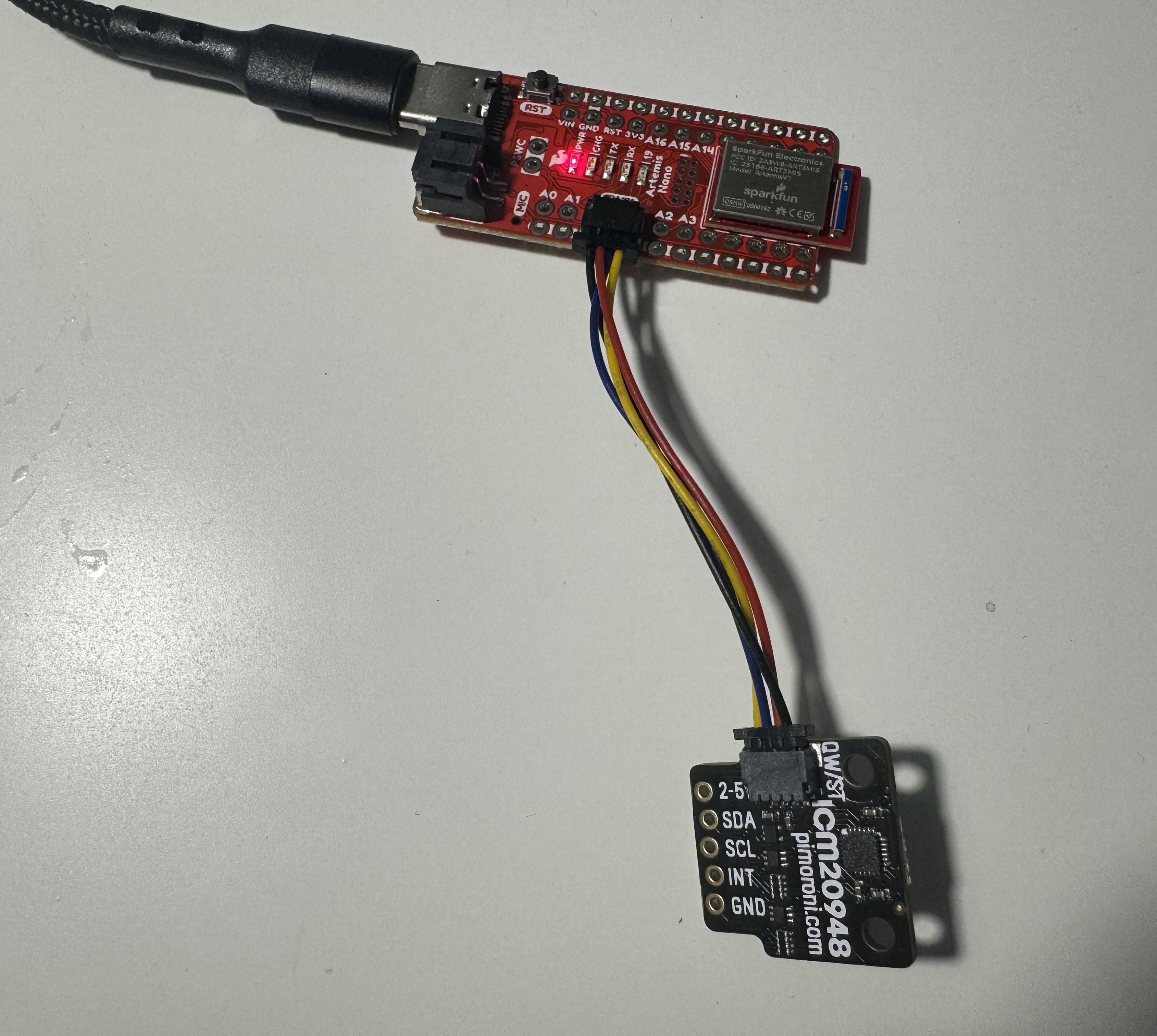
Firstly, it should be connected to the Artemis with wire like shown below.

IMU Example Code

We can run the Example1_Basics in the IMU library, where the results are shown in the video. It can be observed from the serial monitor that the values of accelerometer and gyroscope will vary if the position of IMU is changed.

AD0_VAL definition discussion

The AD0_VAL definition in the code represents the logic level of the address pin AD0 on the IMU breakout board. According to the connection of this pin (either grounded or pulled high), we need to set AD0_VAL carefully. If AD0 is connected to ground, it is required to set AD0_VAL to 0. If AD0 is connected to VCC (pulled high), we should set AD0_VAL to 1.

Start-up Blink

To visually indicate the start-up of the device and the code, the blink function of the internal LED can be added to let people notified.

ACCELEROMETER

As it is taught in the lecture, the equations to convert accelerometer to pitch and roll is:

θ = \( \text{atan2}(ax, az) \)

𝜙 = \( \text{atan2}(ay, az) \)

Therefore, the code can be constructed as below:

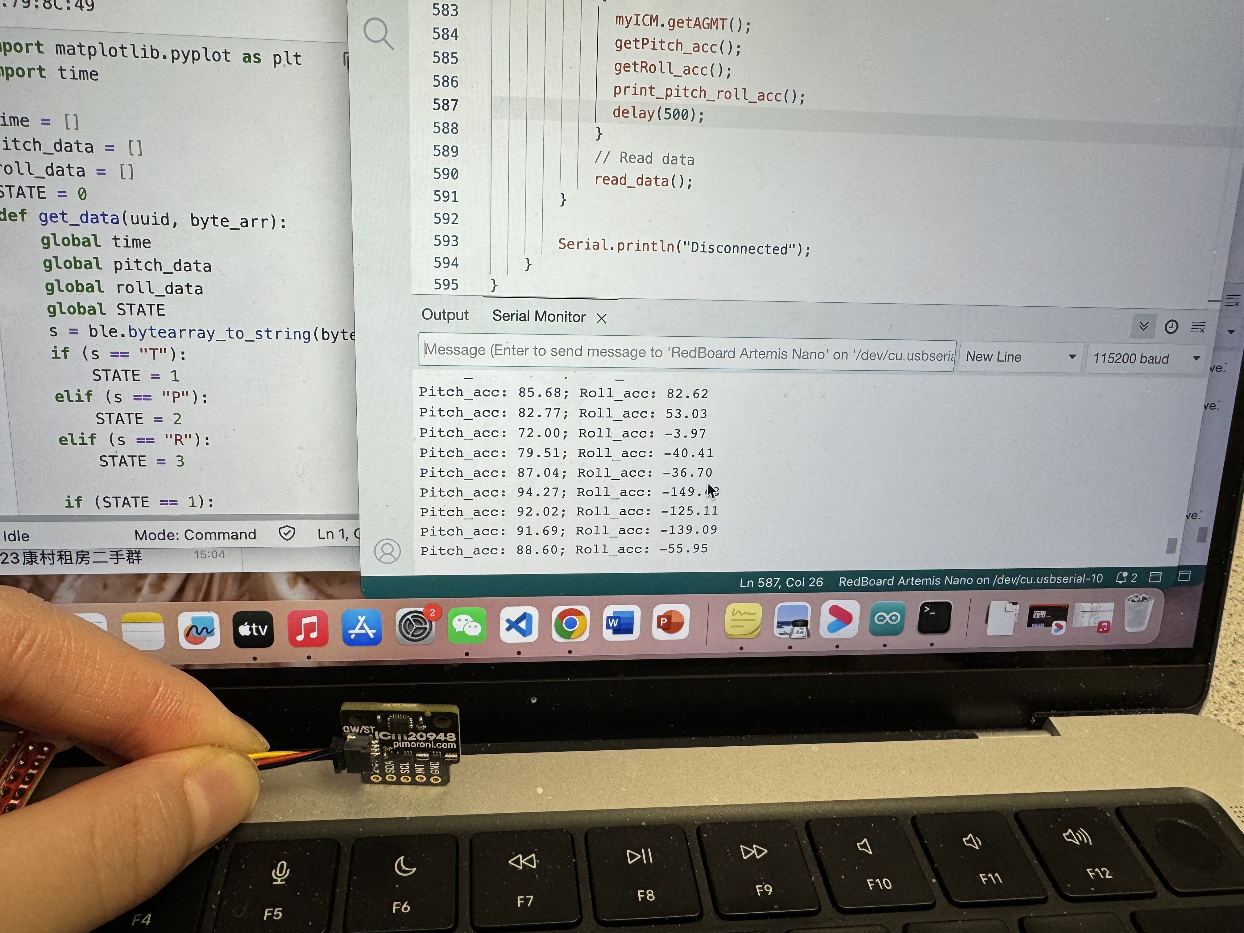
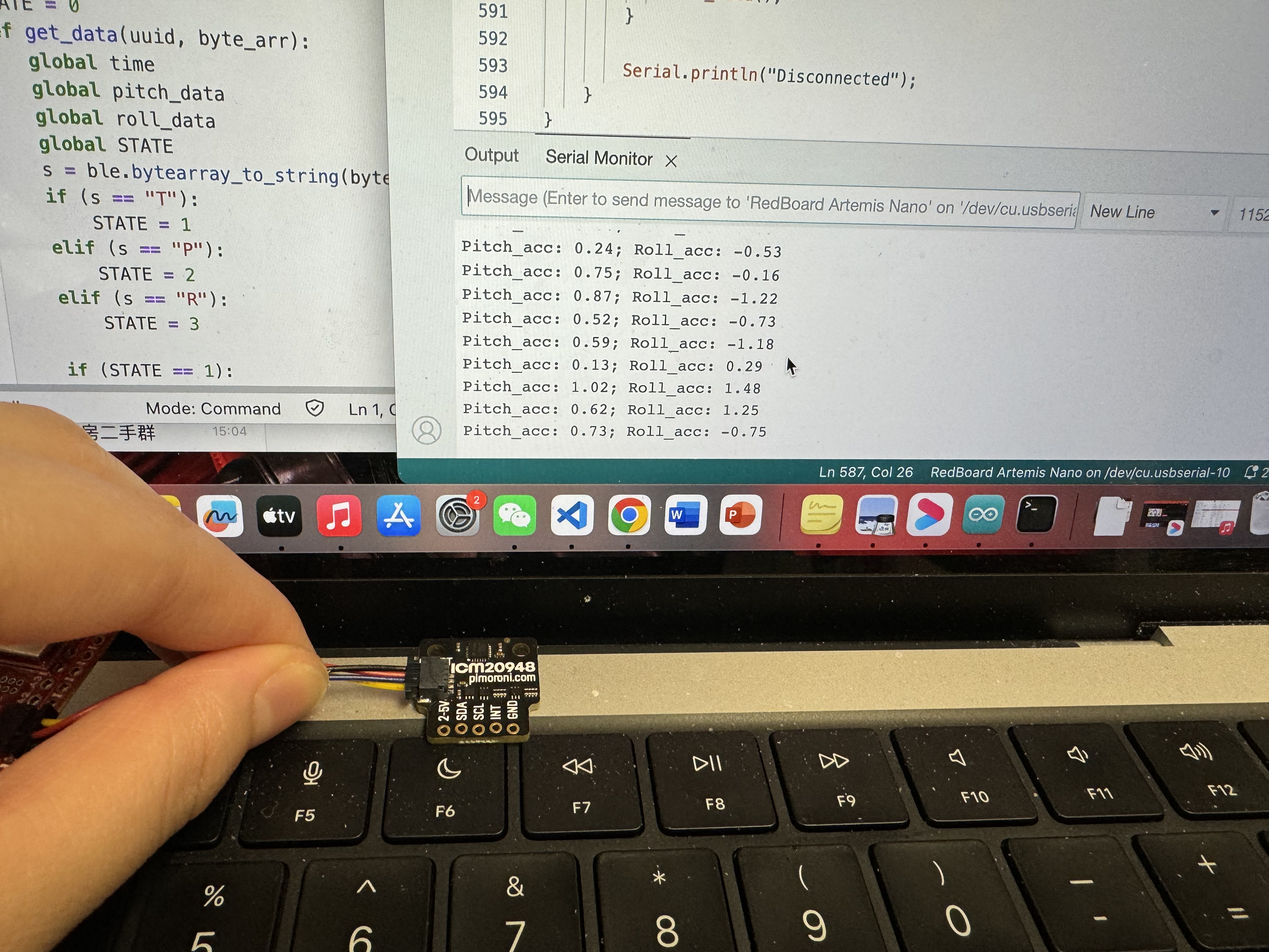
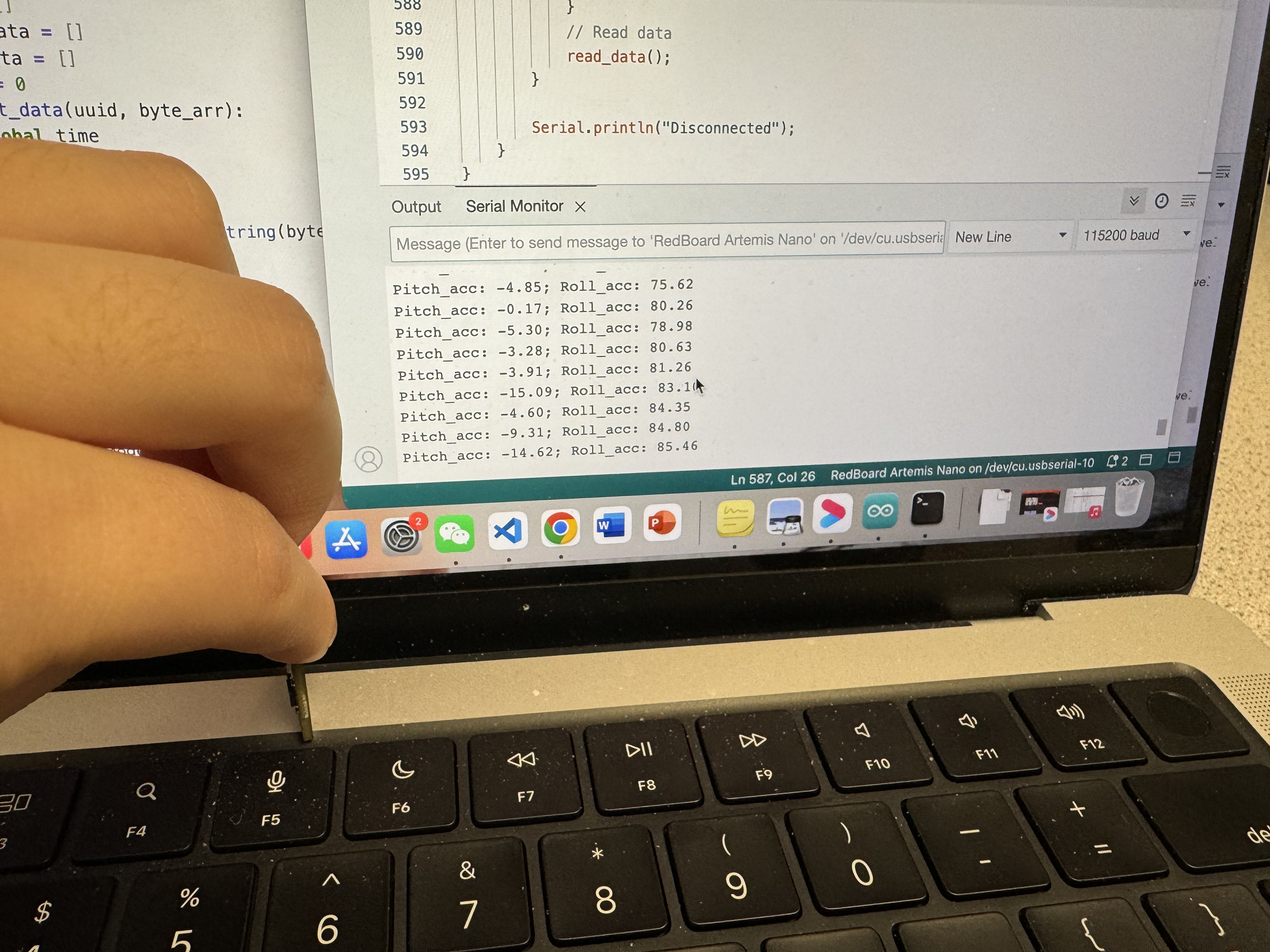
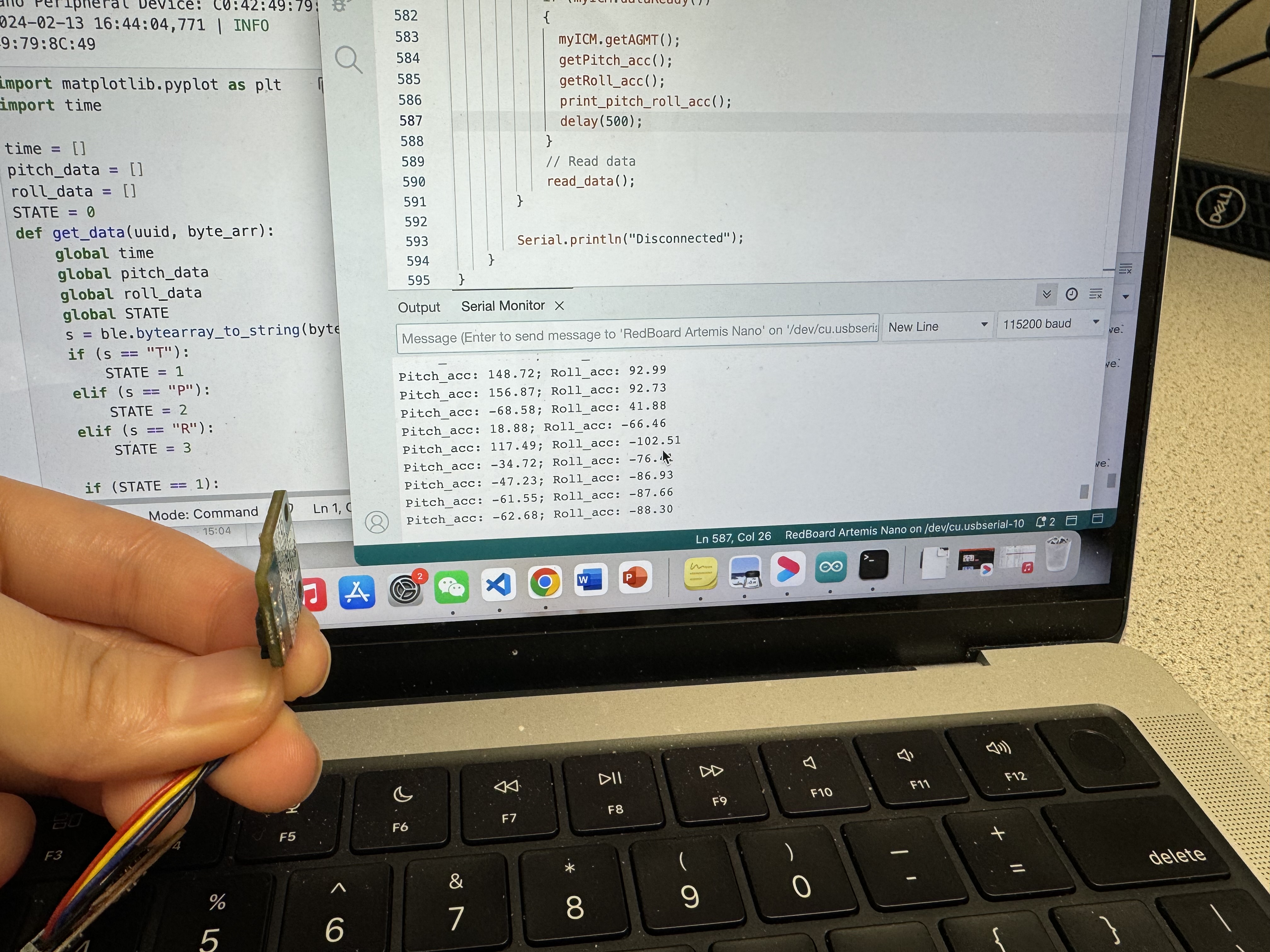
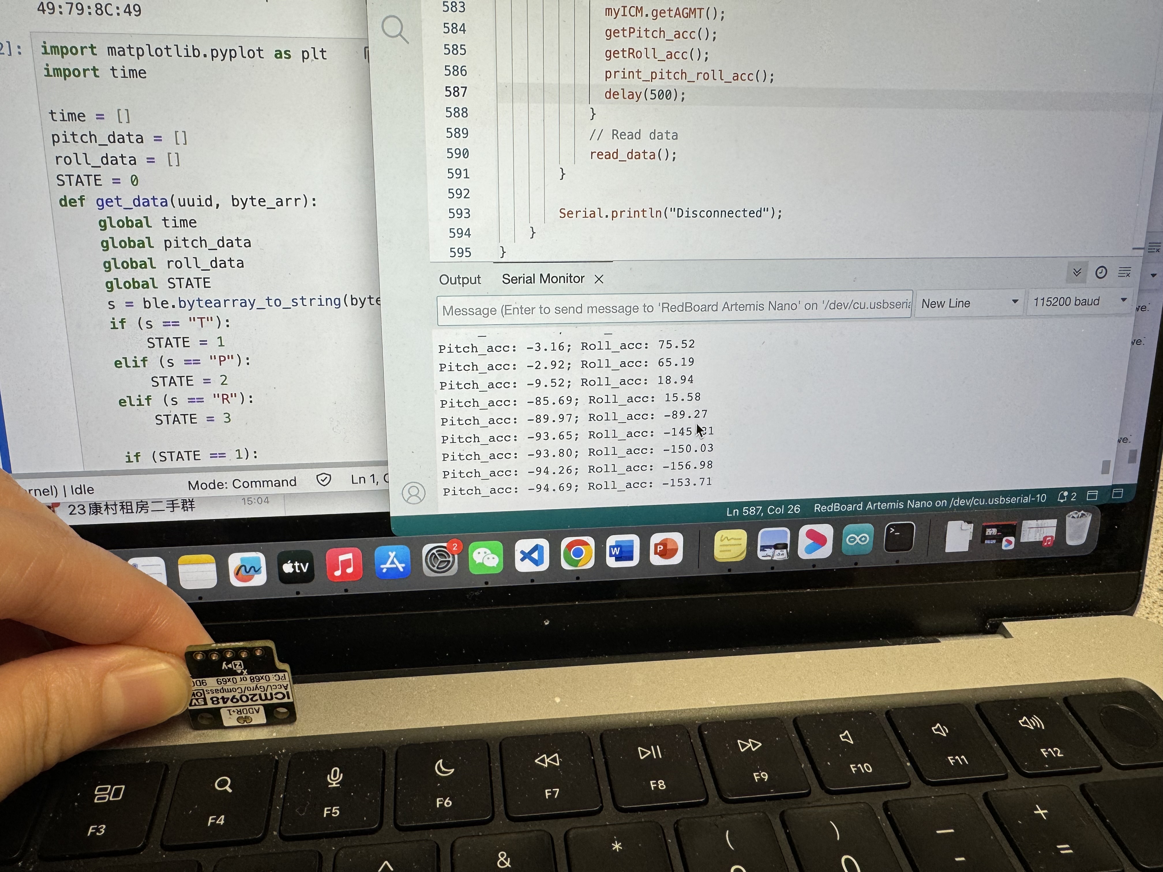
Image of output at {-90, 0, 90} degrees

With the rotation of the IMU, we can get those three different degrees for both accelerometer and gyroscope.

Accelerometer accuracy discussion

When measuring the accuracy with a two-point calibration, it can be concluded that the system is quite accurate. As within the change of 180 degree, the actual change is ranging from 88.6 to -94.69, where the error rate is (183.29-180)/180 = 0.018

Noise in the frequency spectrum analysis

Since the accelerometer module is noisy, it is required to conduct the experiment to find out the cut-off frequency of the low-pass filter that is needed to be implemented into the system. Thus, we can following the guide here to apply Fourier Transform in Python. However, the first thing we should do is to use the command to send pitch and roll data from the Artemis, so the following code is added as a new robot handler in the Arduino file.

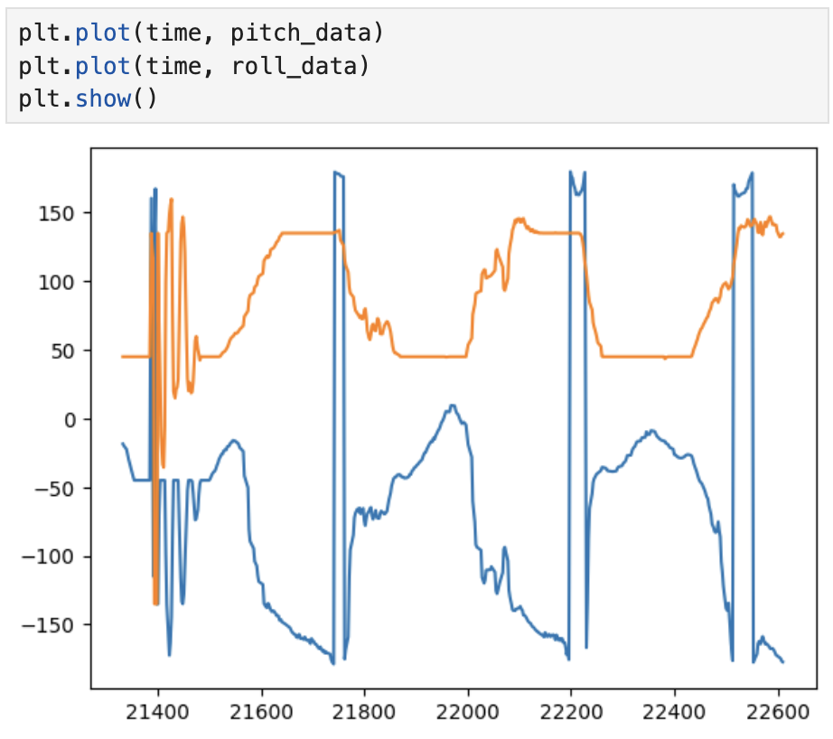
With the data sending from the Artemis, the Python program below is able to receive all those three data arrays and to plot them in time domain.

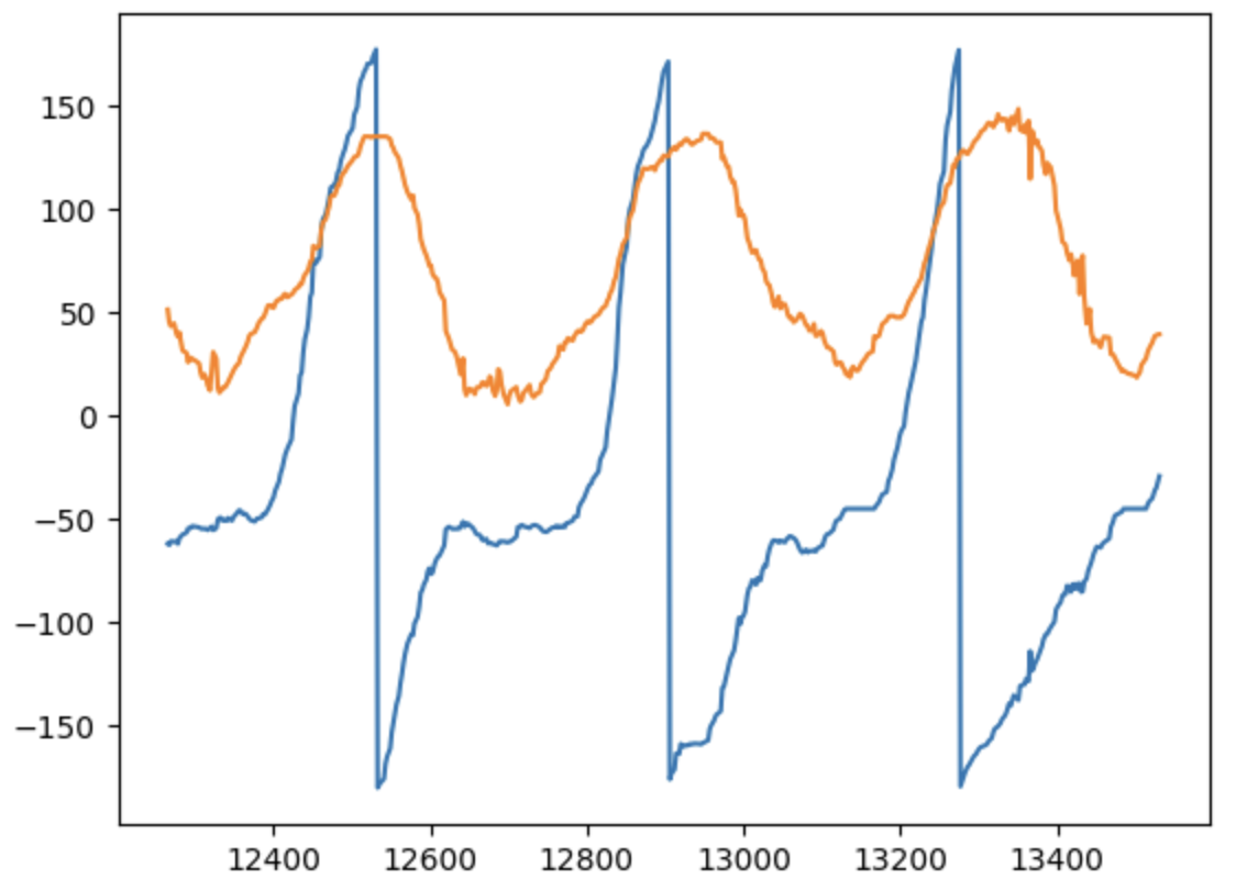
The signal plot in time domain is shown in the figure below.

Fourier Transform

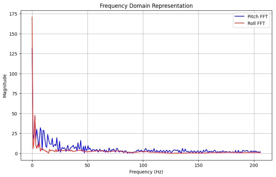
After the IMU data sending and storing process, the Python program should be created to analyze the frequency spectrum, where we can use the time stamps array to calculate T.

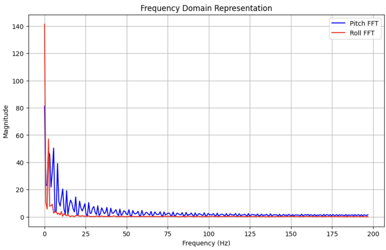
Therefore, the FFT spectrum diagram is acquried and it can be observed that the cut-off frequency should be determined as 10Hz.

According to the equation:

\( \alpha = \frac{T}{T + RC} \)

\( f_{c} = \frac{1}{2\pi RC} \)

Hence, the alpha value of the low pass filter can be calculated as alpha = 0.132 and the low pass code is as below.

The time-domain and frequency-domain diagram are displayed seperately as following. Furthermore, it can be concluded that high-frequency noises have been filtered out to enhance the accuracy of the system, which ensures the robustness of the robot in the future lab.

GYROSCOPE

Pitch, roll, and yaw results

We can also calculate the pitch, roll and yaw based on the gyroscope.

The results are shown in the attached video, where we can observe that the data calculated from the gyroscope will drift more, while they have lower noise than from the accelerometer.

Complementary filter

In the complementary filter, the stability of accelerometer and the fast response of gyroscope can be combined to make the system perform better.

SAMPLE DATA

As instructed, all the redundant components in the main loop should be removed, including delay(), Serial.print().

Moreover, the START_RECORD and STOP_RECORD are added to the current commands.

Time-stamped IMU data in arrays

Similar to the GET_IMU_DATA command, the Python code is shown below.

Speed of sampling discussion

In this circumstance, the time step T can be printed through the Jupyter Notebook, which indicates the speed of data transmission.

Demonstrate 5s of IMU data

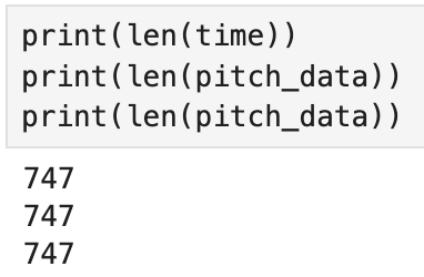
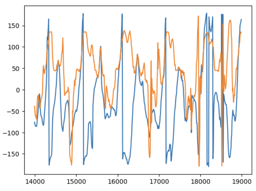
It can be seen that all the array size for IMU sending data within the 5 seconds are 747. Also, the time-domain diagram is shown on the right.

RECORD A STUNT

Record a video showing the behaviors of the robot, which helps establish a baseline for further lab. It is observed that the car can move swiftly with the remote_controlled panel.

DISCUSSION

In this lab section, the IMU module is introduced for analyzing the position of the robot. With the implementation of the accelerometer and gyroscope, the parameters of pitch, roll and yaw can be better calculated, ensuring system accuracy, which is beneficial for further in-depth learning.