INTRODUCTION

This lab section is to implement the PID control to the motors according to the distance from the wall. The BLE is used to store the data and debug the system.

PRELAB

Parts Required

• 1 x R/C stunt car
• 1 x SparkFun RedBoard Artemis Nano
• 1 x USB cable
• 2 x Li-Po 3.7V 650mAh (or more) battery
• 2 x Dual motor driver
• 2 x 4m ToF sensor
• 1 x 9DOF IMU sensor
• 1 x Qwiic connector

BLE

First, I created these arrays to store the data that needed to be transferred to the laptop for analysis through the Bluetooth.

Also, I use these command to start the PID motion control on the robot through BLE:

Hence, with the data sent through the channel, it can be received by the laptop and plot in the figure by the following code. The first block is for PID motor input and TOF distance vs time, and the second block is for plotting each PID component, which helps debugging.

LAB TASKS

P/I/D discussion

As it is stated in the lab section, the PID controller is comprised of three part, propotional, integral and derivative. Therefore, the equation can be represented as:

$\text{correction}=K_p\cdot \text{error}+K_i\cdot \text{integral error}+K_d\cdot \text{derivative error}$

The proportional gain, Kp, adjusts the current error (the gap between the desired and actual values) in proportion to its magnitude. A higher Kp intensifies the corrective action, yet it may lead to instability or overshooting.

The integral gain, Ki, addresses accumulated past errors. It amplifies the corrective action when the error persists over time, but excessive Ki values can result in overshooting or weaving due to the gradual reduction of accumulated errors.

The derivative gain, Kd, anticipates future errors by assessing the rate of error change. It serves as a damping mechanism to minimize overshooting and moderate the speed of corrective actions, although it may also amplify noise.

Range/Sampling time discussion

To make sure that there will be valid data for each loop of the TOF distance reading, the following line is put inside the function pid_position_tof(), but it will delay a lot of the sampling time and make the system unstable. Consequently, I delete those lines. However, if it is deleted, the data might not be valid due to the low frequency of the TOF sensor reading, so there is a problem that will be fully illustrated in next section.

Implementation

To implement this, the case PID_POSITION_CONTROL is created to start that recording function. After recording certain amount of the PID sample data, which is 500 in this situation, it will begin to send data through BLE.

Where the funtion pid_position_tof() for calculation the motor control signals is shown below:

Therefore, with the notification handler, the data can be stored in the array in Python through the command ble.send_command(CMD.PID_POSITION_CONTROL, "0.1|0.1|0.5|304"), where the PID parameter and the target distance can be modified by changing the numbers in"0.1|0.1|0.5|304".

Graph data results

The movement of the robot with PID controller is shown in the video, where the car distance from the wall is set to 304mm (1ft).

And when the parameter Kp is increased, the result is shown below:

Additionally, the data plot in the diagrams indicates the process of the PID control, which will be demonstrated as follows

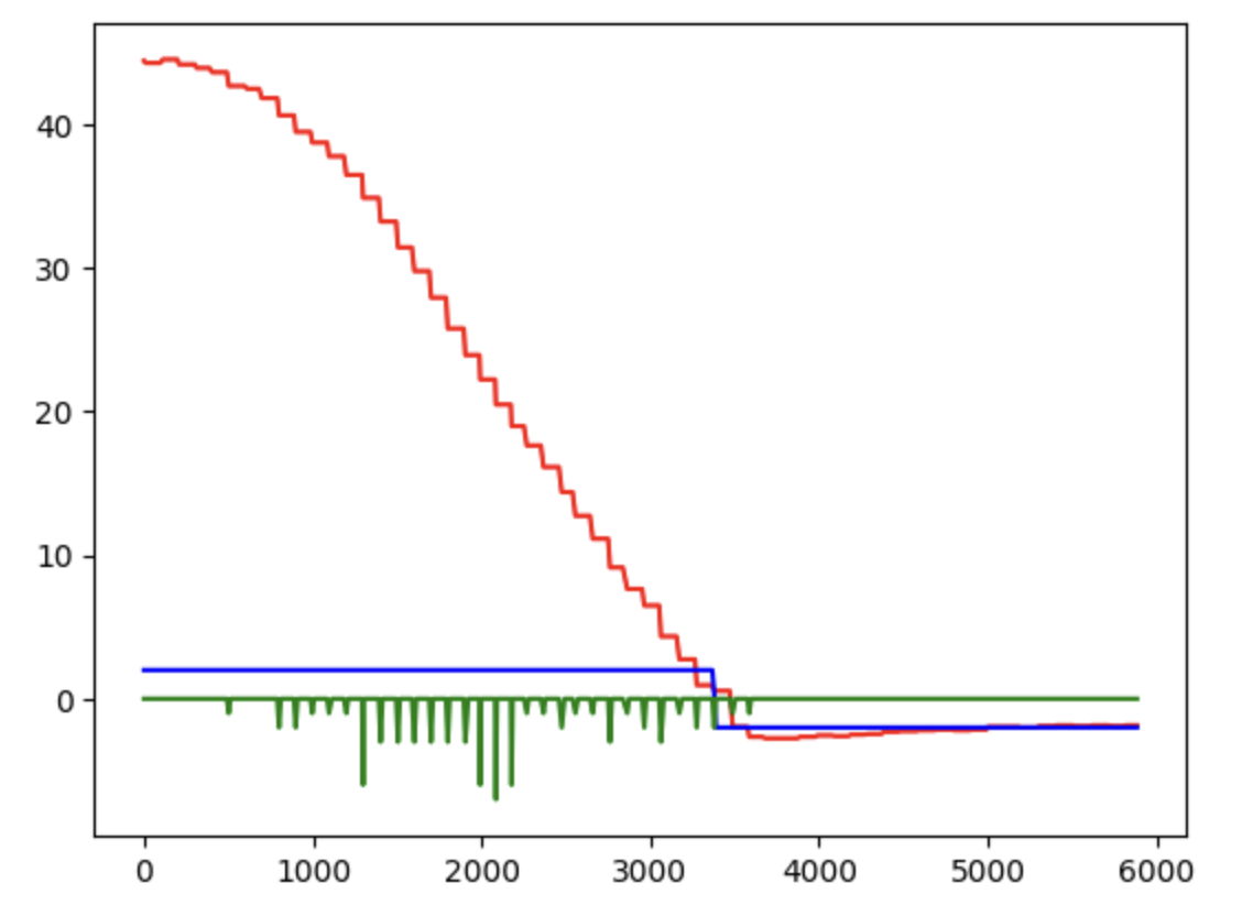
When Kp = 0.05, Ki = 0.02, Kd = 1, the diagram is shown below:

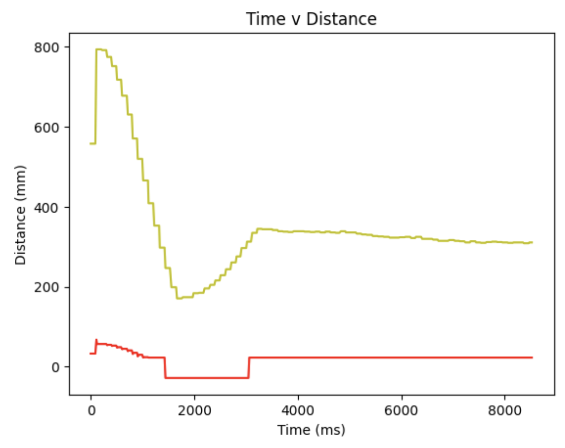
When Kp = 0.1, Ki = 0.01, Kd = 0.8, the diagram is shown below:

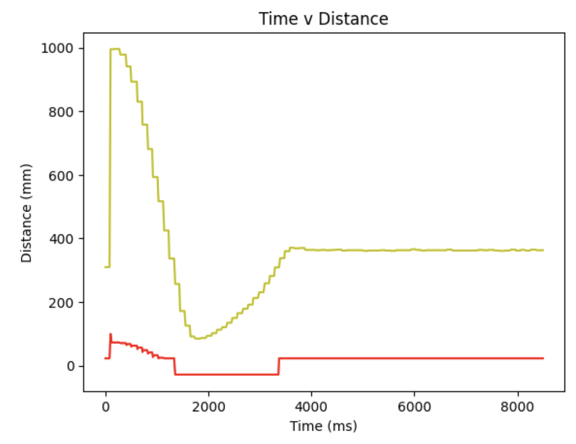
When Kp = 0.1, Ki = 0.005, Kd = 1, the diagram is shown below:

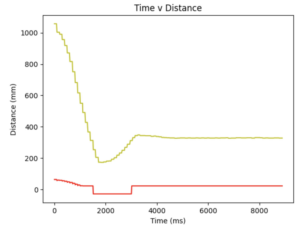
When Kp = 0.08, Ki = 0.005, Kd = 1, the diagram is shown below:

Furthermore, each PID component is also sent to the laptop for analyzing, which is beneficial for debugging.

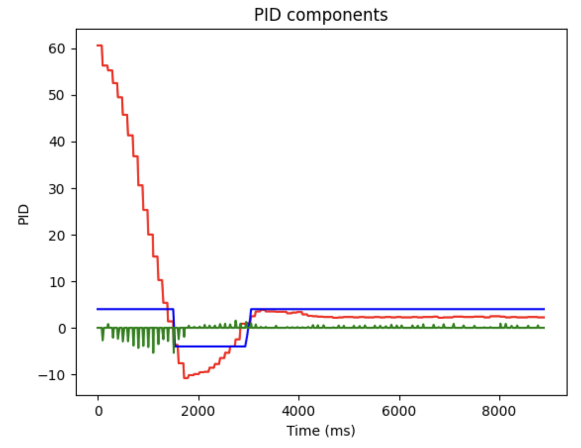
From all the figures above, it can be concluded that only with propotional term the oscillating waveform of motor input will be obstained, so the integral and derivative terms should be added as well. Moreover, the D-term controller values shown in figure are discrete, indicating that some of the TOF values are not valid, since the sampling frequency of the sensor is not high enough. Thus, the extrapolation method should be implemented, which will be illustrated in the following section.

Extrapolation

Since the PID loop run time is around 15ms, while the TOF reading is nearly 8ms, the extrapolation should be implemented to ensure the validity of each data in the pid_tof array. Therefore, the function checkForDataReady() can be used for extrapolating data when it is invalid. Also, according to the interpolation equation reprensented:

$y=y_1+\frac{(x-x_1)\cdot (y_2-y_1)}{x_2-x_1}$

We can create the program as below:

Wind-up protection

Wind-up protection is an essential feature of PID controller, particularly in systems susceptible to integrator wind-up. Integrator wind-up arises when the integral component accumulates excessively due to prolonged error conditions, resulting in issues like overshooting, instability, or other undesirable system behaviors. Therefore, the following code can be implemented to eliminate the wind-up problem. With this applied, the integral term will not be too large to calculate.

DISCUSSION

In this lab, we learnt how to implement the PID controller to the motor according to the TOF distance set up. Furthermore, the extrapolation and wind-up protection are demonstrated as well.