INTRODUCTION

After successfully demonstrating the functionality of our Bayes filter in the preceding experiment, our aim is to apply localization to our physical robot. In this particular experiment, we've solely incorporated the update phase of the Bayes filter, as the robot's movement is affected by considerable noise factors like battery level and wheel-floor friction, rendering the motion modeling unreliable.

LAB TASKS

Bayes Filter (Sim)

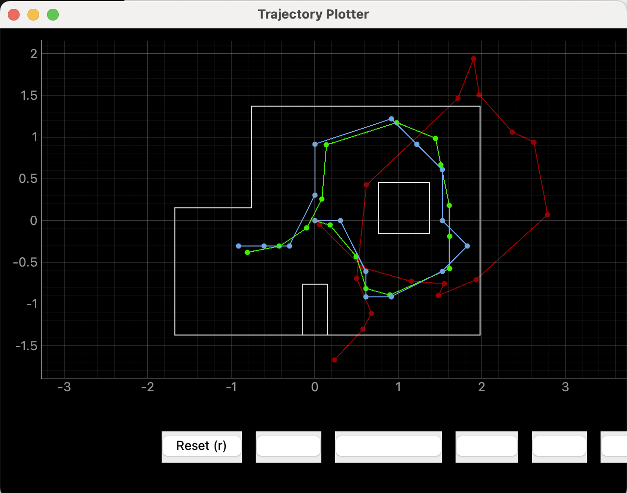
Firstly, we run the given code to display the simulation results, where there are plots for odom, ground truth and belief.

Bayes Filter (Real)

After the simulation, we are requited to run the real robot. Therefore, the LOCALIZATION case is created on the Artemis side as shown on the following. Previously, there was an index error appeared when I run the Python code, and later it was found out that 18 sets of data should be obtained in that function, which indicated that the 0 degree's data was not recorded. Hence, I added the record of that data in the LOCALIZATION case, ensuring I got the first data.

In the main loop of the program, the flag local_on will be checked and the data will be recorded after the increment of the certain angle that is set by the command ble.send_command(CMD.LOCALIZATION, "165|20").

Moreover, in the perform_observation_loop, the code is organized as below, where we send the command and wait for the data transmitted, and then, after 30 secs, we will process the data, since the operation require time to do the rotation. The reason why I implemented asyncio.run(asyncio.sleep(30)) instead of time.sleep(30) is that it can run the localization code on the background, where there is no interference of time.sleep() function.

To receive the record, every 20 degree, the notification handler is implemented, called local_data(uuid, bytearr). With this method, the two parameter can be seperated and stored in different arrays.

Furthermore, we should plot the theoretical dot together with the real position to analyze the performance of the Bayes Filter, where the dots are represented in meters.

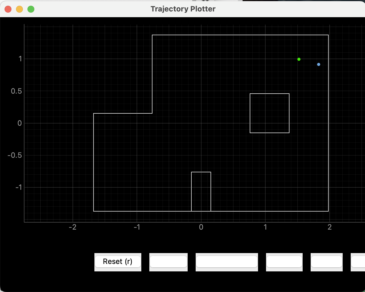
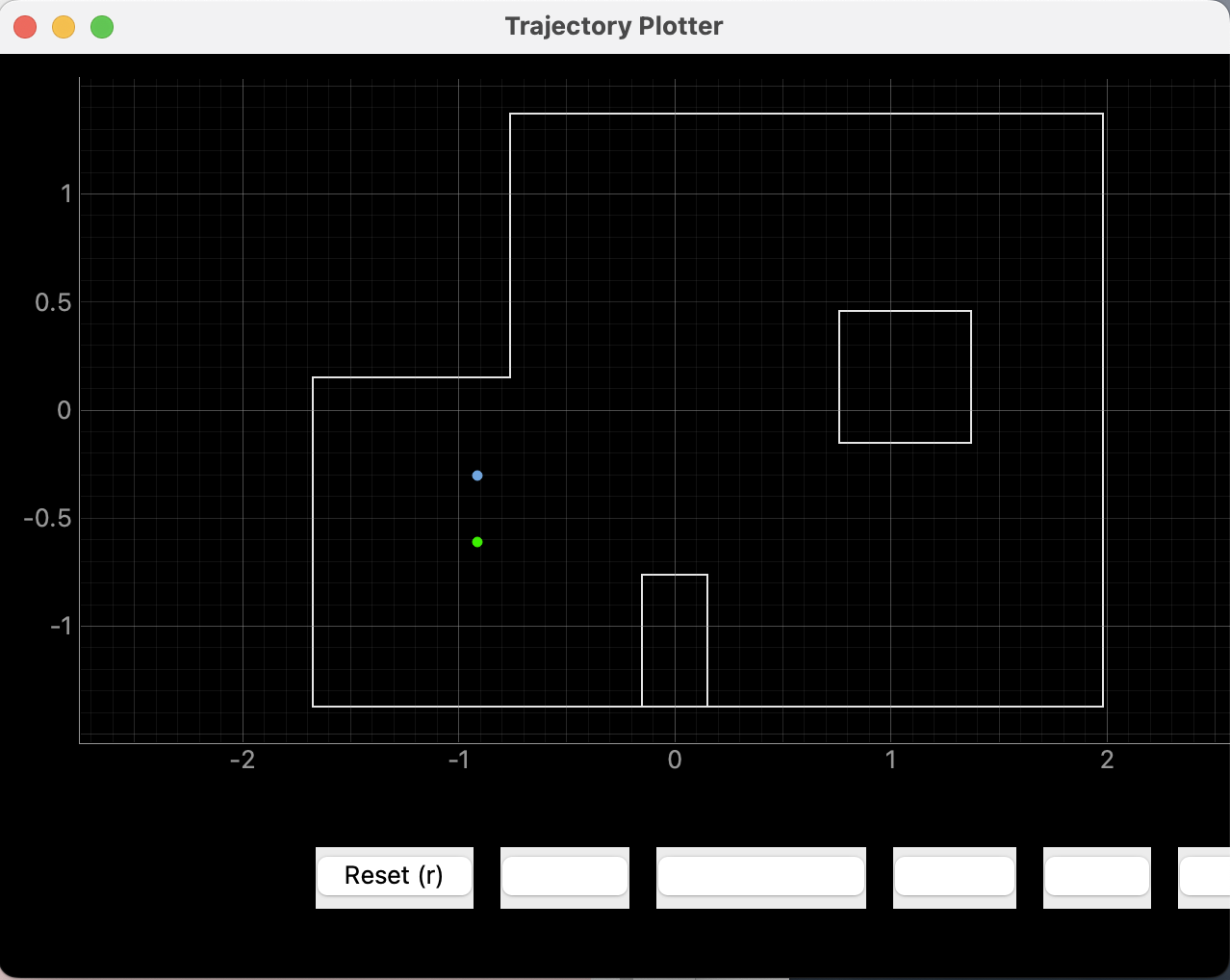
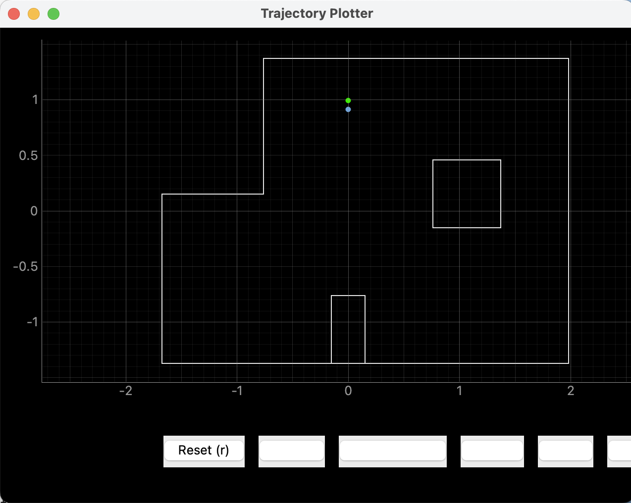
After all the testing, we can obtain the following results, where the green dots stand for theoretical result and the blue dots indicate actual position coordinates.

Position (-3, -2):

Position (0, 3):

Position (5, -3):

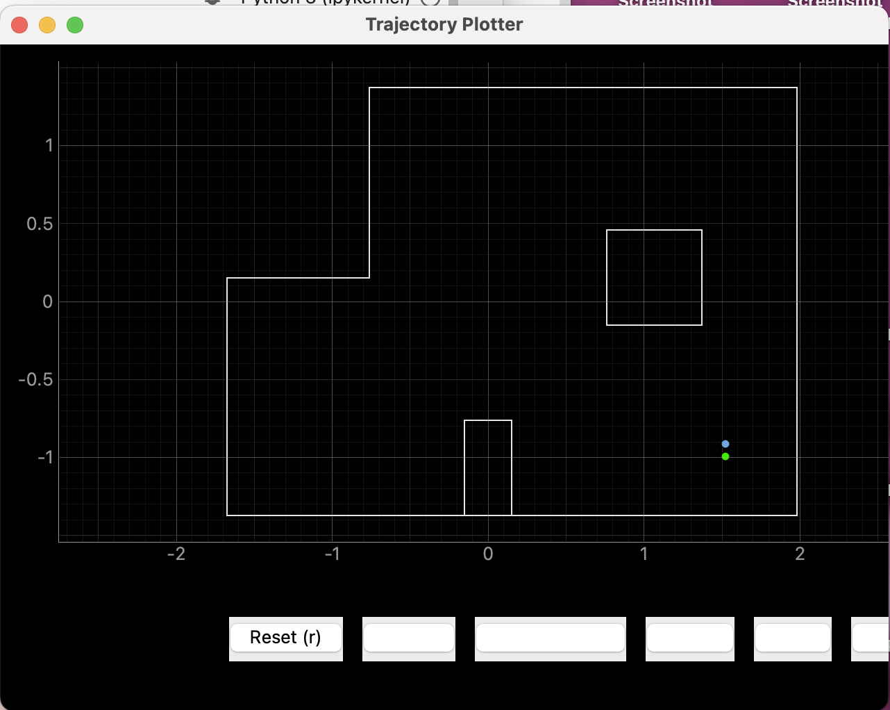
Position (5, 3):