INTRODUCTION

The purpose of this lab is to implement grid localization using Bayes filter.

--------------------------------------------------------------------------------------------------------------------------------------

Prelab

Background

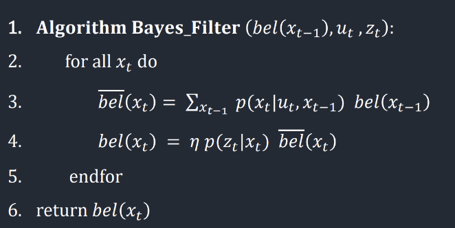
The following figure shows the background information of the Bayes Filter. Additionally, according to the lab instructions, the Python code consists of several modules, which is Compute Control, Odometry Motion Model, Prediction Step, Sensor Model and Update Step.

In essence, each cycle of the Bayes filter involves two main stages:

During the prediction phase, uncertainty in the belief typically increases, while during the update phase, uncertainty decreases. The belief formed after the prediction phase is commonly known as the prior belief. For further details, please see lectures 16 and lecture 17.

LAB TASKS

Concerning the Implemetation of the Bayes Filter, we will follow the lab instruction downloaded from the website.

Compute Control

The forecasting phase depends on control data obtained from the robot, acquired through the odometry motion model. Determining the robot's rotation involves trigonometric calculations based on its current and previous positions. In this stage, I followed the instructions in the comments and adjusted the rotation angles to ensure they fall within the range of (-180, +180) degrees.

Odometry Motion Model

In the next step, we wanted to obtain the probability that the robot would reach some current position x' given the previous position x and odometry values u. Therefore, we first extract the actual control values (representing rotations and translations needed to transition from the previous to the current position) by inputting the current and previous position parameters into our compute_control function. Then, employing a Gaussian distribution, we ascertain the probability that the robot has transitioned to the current position based on the anticipated movement derived from the instructed motion commands. This Gaussian distribution is centered around the expected robot motion computed from the odometry model, with a standard deviation determined by our confidence in the odometry model. Essentially, this function is akin to the probability P(x'|x,u), signifying the probability that the robot has arrived at the current location x' given the previous location x and the movement commands u.

Prediction Step

Now, equipped with all the required values, we are ready to execute the prediction step of the Bayes Filter. Hence, we looped through all the values. In addition, tp speed up the filter, all the grid hexes where the robot is unlikely to be could be ignored, with the threshold of P(robot's prev pos at (x, y, theta)) >= 0.0001.

Sensor Model

In the latter stage of the Bayes Filter, we refined our predicted probability distribution with sensor measurements. To begin, we construct the sensor_model() function. This function operates on a pre-calculated array of true observations for a specific pose in the grid. It computes the probability of each sensor measurement based on the observations recorded by the robot's sensors post-movement. Utilizing the Gaussian function, with the true observation as the mean and sensor_sigma as the standard deviation (representing the sensor model's noise parameter), it generates an array comprising the probabilities. Essentially, this function assesses the likelihood that the sensor observations align with the true observations for a given pose in the grid.

Update Step

To update the step, we nested three for loop to do the calculation so that the belief value of each potential position can be calculated through each iteration. Thus, the function program is listed below:

Results

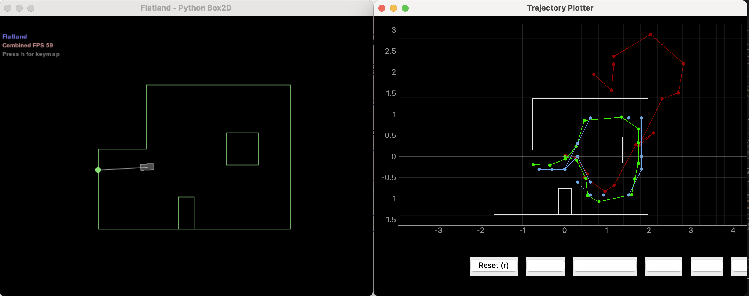
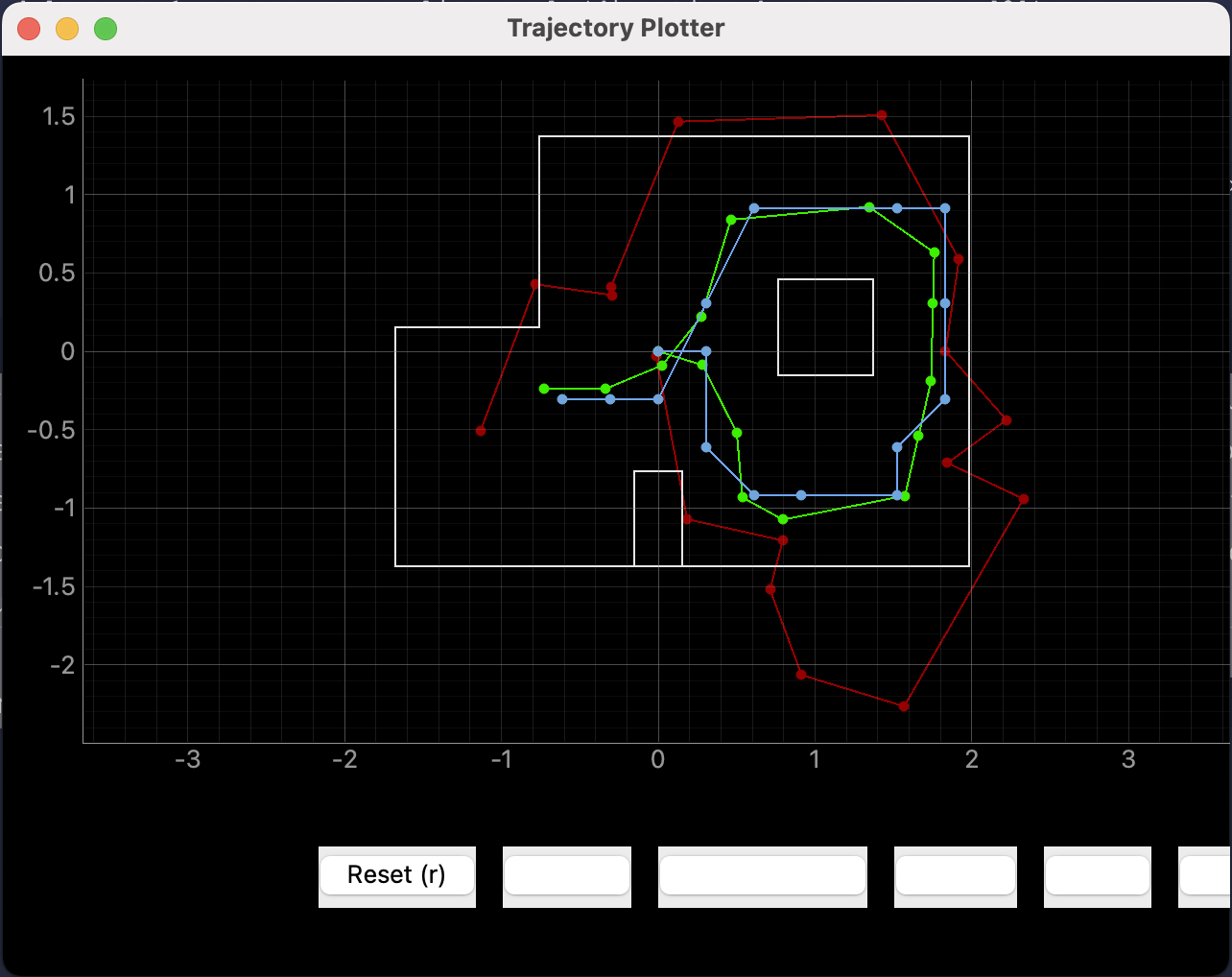
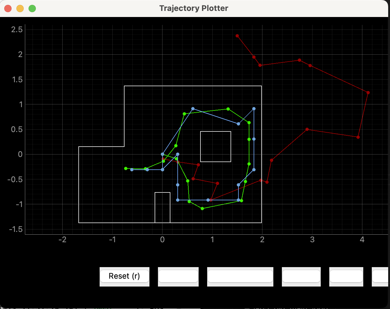
Consequently, with all the above design and implementation, the following results can be obtained, where the red line represents for the odometry values, the green line stand for the true positions and the blue line indicates the belief values.

This video display the process of the licalization:

Furthermore, the following is the data output during that process.